
This post presents key concepts in statistics that describe or summarize the characteristics of a sample or a dataset, thus enabling successful exploratory data analysis: central tendency, dispersion/variability, distribution and correlation.
Central Tendency #
Central tendency identifies the central position within a dataset. It is commonly measured by the arithmetic mean, the median, and the mode.
Consider a sample containing prices of dresses: DressPrice[28,20,34,19,24,27,28,19,31]
Arithmetic mean (or simply mean) is the sum of values in a sample divided by number of items in the sample = 230/9 = 25.56
Mode is the value that appears most often in a sample; a sample with more than one mode is called multimodal. This sample has two modes – 28 and 19 – and is referred to as bimodal.
Median is the value in the middle of a data sample, population or distribution when the data is arranged in increasing order. If the sample has an odd number of data points, then the median is the middle data value when the data is arranged in increasing order. If the sample has an even number of data points, then the median is the mean of the two middle data values when the data is arranged in increasing order.
The new look dataset after rearranging the values is DressPrice[19,19,20,24,27,28,28,31,34] and median = 27.
Dispersion/Variability #
Range is the numerical difference between the largest and the smallest values
First quartile (Q1) is a measure of dispersion that indicates where the lower 25% of the values are located in a sample. It is calculated as the median of the lower half of the sample. Lower half of the DressPrice sample is [19,19,20,24], its median and therefore Q1=(19+20)/2=19.5.
Third quartile (Q3) is a measure of dispersion that indicates where the upper 25% of the values are located in a sample. It is calculated as the median of the upper half of the sample. The upper half of the DressPrice sample is [28,28,31,34], its median and therefore Q3=(28+31)/2=29.5.
Interquartile range (IQR) is a measure of dispersion that indicates where the middle 50% of the values are located. It is calculated as IQR=Q3-Q1, in this case IQR=29.5-19.5=10.
IQR is a very important statistic because it does not include extreme values (outliers). Consequently, it is an adequate measure for eliminating outliers in a dataset
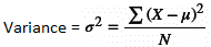
Variance measures how far data points are spread out from their average value; the closer the variance to zero, the more closely the data points are clustered together. Its official formula is:
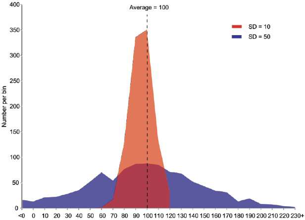
Standard deviation quantifies the amount of variation or dispersion of a set of data values; the lower the value, the closer the data points are to the mean on the dataset. Figure 1 below illustrates the difference between low- and high standard deviation.
By JRBrown – Own work, Public Domain, https://commons.wikimedia.org/w/index.php?curid=10777712
Accessed on 10 May 2022
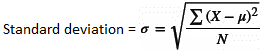
The formula for standard deviation is:
Variance is identical to the square of standard deviation and hence expresses “the same thing” (but more strongly).
Distributions #
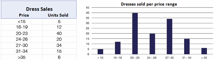
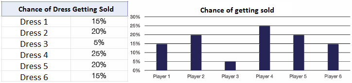
Frequency distribution: table or graph displaying the frequency of various outcomes in a sample. It summaries the distribution of values in the sample. See example in Figure 2.
Probability distribution: a graph or table that depicts the likelihood of all potential outcomes in a sample. It provides the probabilities of occurrence of different possible outcomes in an experiment. Figure 3 shows probability distribution of data from Figure 2.
Sampling distribution: probability distribution based on a random sample of a dataset
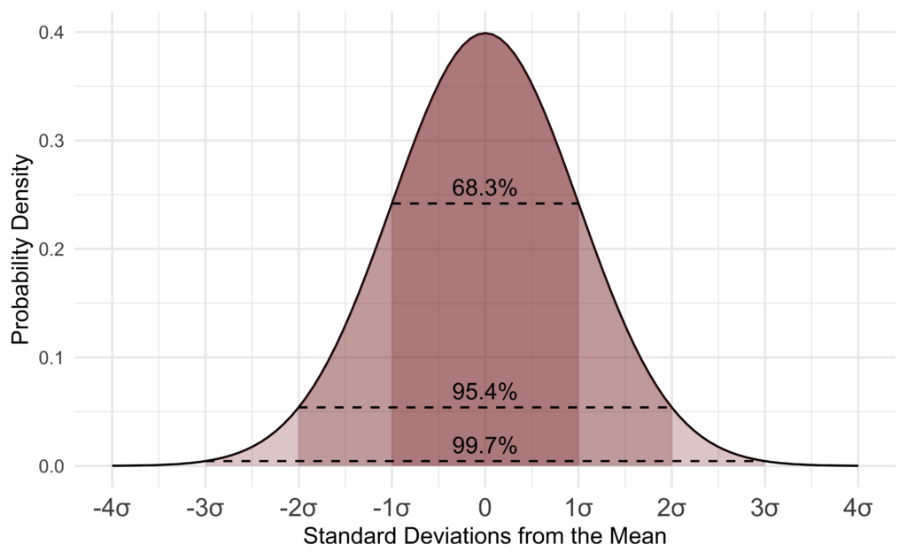
Normal (or Gaussian) distribution represents data that occurs where most values are the same as the mean and only a few are found at the extremities. Approximately 99.7% of the values are within three standard deviations of the mean, while 95.4% are within two standard deviations of the mean and 68.3% are within one standard deviation of the mean. Normal distribution has the same mean, median, and mode. The area under the normal distribution curve is equal to one. See Figure 4 below.
D Wells, CC BY-SA 4.0 https://creativecommons.org/licenses/by-sa/4.0, via Wikimedia Commons
Accessed on 10 May 2022
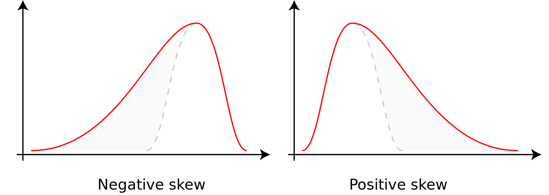
Skewness measures how data is distributed around the mean; it can indicate potential bias in a dataset. See Figure 5
By Rodolfo Hermans (Godot) at en.wikipedia. – Own work; transferred from en.wikipedia by Rodolfo Hermans (Godot)., CC BY-SA 3.0, https://commons.wikimedia.org/w/index.php?curid=4567445
Accessed on 10 May 2022
- Negative skew: the majority of the values exist on the right side of the curve, and the mean is less than the median and mode
- Positive skew: the majority of the values exist on the left side of the curve, and the mean is greater than the median and mode
Correlation #
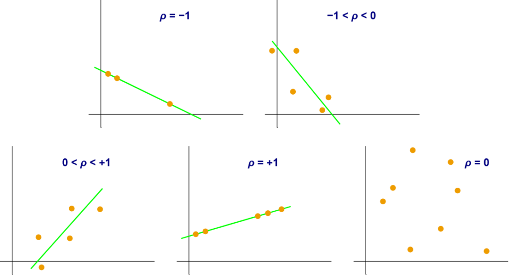
Pearson correlation coefficient a measure of the linear correlation between two variables. +1 indicates the values of the variables move in the same direction in perfect unison, -1 indicates variation in perfectly opposite directions, and zero indicates no correlation at all. See Figure 6 below.
Kiatdd, CC BY-SA 3.0 https://creativecommons.org/licenses/by-sa/3.0, via Wikimedia Commons
Accessed on 10 May 2022
IMPORTANT: Correlation does not imply causation, i.e., two events happening together does not necessarily mean there is a cause-and-effect relationship.
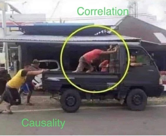
Source: https://twitter.com/VirginiaBuysse/status/1420350036144177152
Accessed on 10 May 2022


