
Business Problem #
As a marketing executive for an FMCG company you are required to design the budget for the next advertising campaign for TV, radio, and newspapers for a certain product. After careful consideration you decide to use a machine learning model that can predict the sales volume for the different media mixes to evaluate budget proposals.
Since the solution involves modeling data with known input/output mappings (values for budgets for TV, radio and newspaper as input and the corresponding values for sales as output), this is a supervised learning problem. Specifically, this is a linear regression problem because the values are numeric.
Gather Data #
Download the dataset (historical data) comprising advertising budgets and the corresponding sales for each of the advertising channels for the last 200 campaigns from https://www.statlearning.com/s/Advertising.csv. Open it and study its structure – number of columns, number of rows, types of data (see Types of Data), range of value, etc.
Download proposed budgets (new data/prediction data/production data) from https://github.com/sdfungayi/advertising-model/raw/main/Advertising_Proposals.xlsx. Notice that the new data is within the range of values in the training set (otherwise model predictions will be wild) and has data columns of the same type as the historical data.
A dataset is a simple, flat table containing historical data for building a machine learning model. In supervised machine learning columns are divided into a set of descriptive features and a single target feature also called a label. In the Advertising dataset the columns “TV”, “radio” and “newspaper” are the descriptive features and the column “sales” is the target or label.
Machine Learning Platform #
Orange Data Mining, a free point-and-click, drag-and-drop, software for machine learning will be used. Orange was selected because it is easy to use and easy to understand.
Download the latest version for your operating system from https://orangedatamining.com/download and install it; the Windows file is over 400MB in size.
Optional but recommended: Quickly learn how to use the software here: https://www.youtube.com/channel/UClKKWBe2SCAEyv7ZNGhIe4g
Workflow #
To get the maximum benefit from this section the reader is advised to attempt to build the workflow by following the steps given below or by referring to the workflow image before running the Orange workflow file contained in the ZIP file below.
Download the Orange workflow file (ows) and image from https://github.com/sdfungayi/advertising-model/raw/main/Advertising%20Workflow.zip.
Load Data #
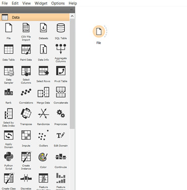
Start Orange Data Mining software and add the widget File from the Data tab to the canvas by double-clicking it or by dragging it to the canvas, Figure 1 below.
Double-click the widget File and navigate to the folder where the file Advertising.xlxs is located and import the dataset into the software. Save your work as often as possible to avoid loss.
Open the widget File on the canvas by double-clicking it and study the summary of the dataset. Verify that the data displayed in Orange matches that in the Excel file – steps 1 and 2 in Figure 2 below.
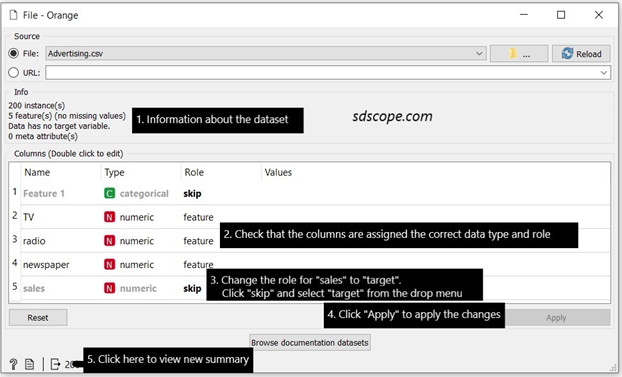
Set the role for the column “sales” to “target” and view the new summary of the dataset – steps 3, 4 and 5 in Figure 2 above.
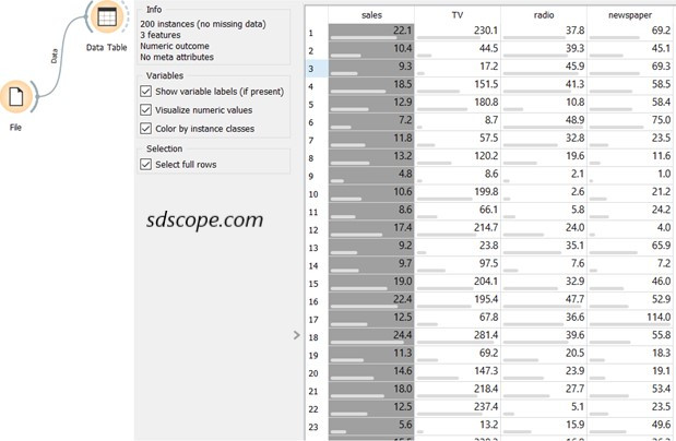
Add the widget Data Table and connect it to the File widget, Figure 3. Open Data Table and view the features of the dataset that will be used in building the model: 3 features and a numeric outcome/target. Notice that the first column, marked “skip” in Figure 2, will not be used for modeling; this is because it contains row identification and no data about the problem.
Select a Model Evaluation Approach #
Model evaluation is the process of determining the capacity of a model to make useful predictions on new, never-before-seen data. See Predictive Modeling (Supervised Learning): Introduction and Model Evaluation.
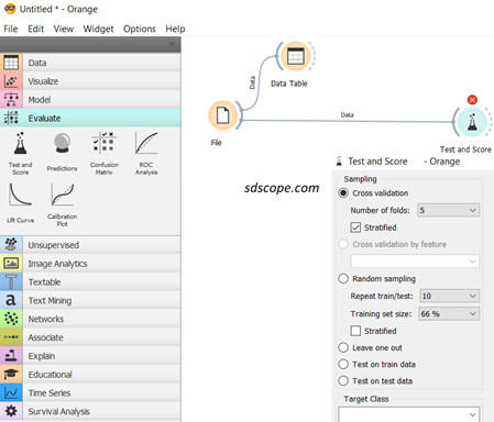
In Orange software open the Evaluate tab and add the Test and Score widget to the canvas; the Test and Score widget calculates the performance of each model built during the process.
Connect the widget to the File widget, open it and set sampling to “Cross validation” and “Number of folds” to 5, Figure 4 below.
k-fold cross validation is one of the several model evaluation techniques and is regarded as the gold standard for model evaluation and for handling the problem of “overfitting”. Overfitting occurs when a model learns a dataset too intricately to be useful on any other dataset since no two datasets are exactly identical in the real world, see Model Evaluation.
Establish a Baseline Performance #
It is impossible to know in advance which machine learning algorithm will perform the best for a given problem; the only way is to try as many algorithms as possible. This is known as “No Free Lunch Theorem”. So a baseline performance must be established: algorithms that perform better than the baseline will be carried forward to the next stage while those that perform worse this will be immediately discarded.
In Orange open the Model tab and add the Constant widget and connect it to the Test and Score, Figure 5 below. For a regression task Constant establishes the baseline performance by predicting the mean of the training dataset.
Create Models #
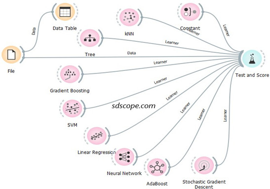
Add all the widgets in the Model tab to the canvas and connect them to Test and Score.
Delete the widgets that do not connect to Test and Score with a solid line (for example Stacking, Load Model and Save Model) or that connect with a solid line but trigger a red warning in Test and Score (for example, Logistic Regression, Naïve Bayes and Random Forest) because they do not apply for this problem. See Figure 5 above.
Select Model #
Model selection is the process of determining the model with the best performance against an evaluation metric that was selected during the business problem definition stage (see Model Selection). The key regression evaluation metrics are Mean Square Error (MSE), Root Mean Squared Error (RMSE), Mean Absolute Error (MAE) and Coefficient of Determination also known as R-Squared (R2), see Performance Metrics.
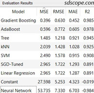
Open Test and Score and study the evaluation results, Figure 6. In this exercise it is assumed that MSE (mean squared error) was the selected evaluation metric. Neural Network performs worse than Constant and should be dropped from further consideration (this action is irrelevant in this exercise since no further experimentation will be done on algorithms).
Click the heading “MSE” to sort the results so that the lowest MSE value goes to the top. Gradient Boosting has the lowest MSE and is thus selected to make predictions on new data.
Save the Model #
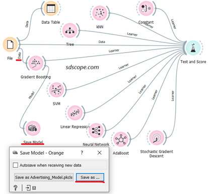
Add the widget Save Model from the Model tab and connect it to the output of Gradient Boosting. Also connect the output of File to Gradient Boost as shown in Figure 7 below.
Open Save Model and give the model a name. Notice that the model is simply a file generated by running an algorithm over a set of data to recognize certain types of patterns in the data.
Make Predictions #
Also referred to deployment, scoring, putting the model into production, etc, this step involves using the saved model to reason over new, never-before-seen data and make predictions which will be used to inform or automate business decisions about those data.
Open a new workflow in Orange software (in the menu click File then New) and give it a name.
Add the widgets File and Save Data from the Data tab, the widget Predictions from the Evaluate tab and the widget Load Model from the Model tab to the canvas.
Connect the widgets as shown in Figure 8 below.
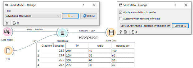
Open Load Model, navigate to the folder where the model was saved and load the model.
Open the File widget and import the file “Advertising_Proposals” which contains new data (several proposed budgets) for which “sales” will be predicted.
Open the Predictions widget; the predictions for each advertising budget proposal are contained in the column “Gradient Boosting”; the predictions can be accessed in Excel in the file specified in Save Data widget.
You can now use the predicted values to inform your selection of a budget proposal.
Emphasis: The new data must be within the range of values in the training set otherwise the predictions would be wild. It must also have data columns of the same type as the historical data.
End #
Congratulations on building your first machine learning model and using it to solve a business problem.
Model Completeness #
Several steps were simplified or overlooked to allow the learner to build their first model in a gentle and fast way. Some of the steps left out are exploratory data analysis, data preparation, residual analysis, model optimization/tuning, AI ethics, performance improvement using ensemble methods, model interpretation, model validation, and model monitoring while business problem definition/identification was oversimplified. These steps are covered in detail in the section “Predictive Modeling“.
Key Takeaways #
- It is possible to build and use a machine learning model without writing a single line of code
- A dataset for a supervised machine learning problem consists of a set of descriptive features and a single label/outcome
- The goal of machine learning is find the model that generalizes well on new data
- A train set is used to create a model and a test set is used to validate the model
- It is not possible to know in advance which machine learning algorithm will perform the best for a given problem; the only way is to try as many algorithms as possible (No Free Lunch Theorem)
- Baseline performance provides a reference point from which to compare other machine learning algorithms
- A machine learning model is simply a file generated by running an algorithm over a set of data to recognize certain types of patterns in the data
- Prediction data must be similar to the training set in terms of both structure and range


