
A performance metric is a number that is used to determine how well a machine learning model generalizes on new data. It typically compares the predictions the model makes on a hold-out set against the expected values in the hold-out set.
Performance metrics are the primary determinant in model selection. They are also used guide in improving the performance of a model.
Classification Metrics #
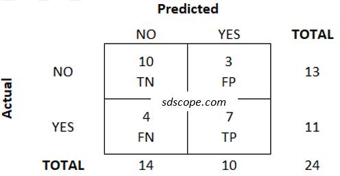
Suppose we had a test set containing 24 records made up of 13 that have a label NO and 11 that have a label YES, and the validation process produced the following results (the outcome of primary interest is labeled “positive” and the other “negative”):
– 7 records that were positive in the test set were correctly identified during validation: these are known as true positives (TP),
– 10 records that were negative in the test set were correctly identified during validation: these are known as true negatives (TN),
– 3 records that were negative in the test set were incorrectly identified as positive during validation: these are known as false positives (FP), and
– 4 records that were positive in the test set were incorrectly identified as negative during validation: these are known as false negatives (FN)
Understanding what these results mean in the real world is very important because they are used to derive several important performance metrics, key of which are given below. The choice of metric or set of metrics depends on the use case. For example, more false positives would be preferable in a model for predicting cancer but not so in a churn model for identifying customers to give an incentive to stay.
Classification Accuracy (CA )is the ratio of correct predictions to the total number of predictions.
CA = (TP+TN) / (TP+TN+FP+FN) = (7+10) / (7+10+3+4) = 0.708
CA is a good measure when the target variable classes in the data are balanced or nearly balanced, e.g., 60:40. It should NEVER be used as a metric when the dataset is imbalanced, i.e., when one class is over-represented in the target variable. Assume we had a churn prediction model that predicted every customer as Loyal and a dataset that had 1,000 instances of which only 5 were churn cases. The model would classify 995 Loyal customers correctly and 5 churned customers as Loyal, giving a very high accuracy of 99.5% despite the result being the same as random guessing, i.e., the model would be useless.
Precision is the proportion of positive instances that were correctly predicted. It indicates how confident we are that the instances predicted as positive are actually positive.
Precision = TP / (TP+FP) = 7 / (7+3) = 0.700
The higher the Precision the fewer the false positives.
Recall or Sensitivity is the proportion of actual positive instances which are correctly identified. It indicates how confident we are that the model has found all the positive instances.
Recall = TP / (TP+FN) = True Positive Rate = 7 / (7+4) = 0.636
The higher the Recall the fewer the false negatives.
Specificity is the proportion of actual negative instances which were correctly identified. It indicates how confident we are that the model has found all the negative instances.
Specificity = TN / (TN+FP) = True Negative Rate = 10 / (10+3) = 0.769
Specificity is the exact opposite of Recall. The higher the Specificity the fewer the false positives.
Logarithmic Loss or Cross-entropy, commonly referred to as LogLoss, quantifies how close a prediction probability is to the actual value. While its actual interpretation depends on the use case, in layman terms a lower LogLoss value suggests better predictions. LogLoss is especially useful when the dataset is imbalanced.
F1 Score is the weighted harmonic mean of precision and recall.
F1 = 2 x (precision x recall) / (precision + recall) = 2 x (0.7 x 0.636) / 0.7 + 0.636) = 0.666
In generally, changing Recall affects Specificity; so F1 is a good metric to use if the intention is to maximize the two.
The results also can be presented in the form of a table known as the Confusion Matrix, Figure 1 below, which enables users to more easily determine which data the model may be able to categorize correctly. Though not a performance metric, the Confusion Matrix is a key tool in making business decisions in the real world.
Receiver Operating Curve (ROC) is a plot of the True Positive Rate (Recall) against the False Positive Rate (also interpreted as 1-Specificity) as the prediction threshold is varied from 0 to 1, illustrated in Figure 2 below. [Note: classification predictions are probability scores that are converted into target classes based on a threshold; the value of the threshold depends on the use case]. It is not a performance metric but a tool that enables visual evaluation of a model or models. The closer the elbow of the curve to the top left corner the more accurate the model. The optimal performance is at the elbow of the curve but the ideal point depends on use case. A ROC curve that runs below the random classifier line signifies an inverted selection of the positive class.

Area under ROC Curve, commonly referred to as AUC, is a single number that represents model quality. It measures how well the model separates classes. Potential values range from 0.5 (random model) to 1.0 (perfect separation between the classes). While the right value depends on the use case, generally AUC greater than 0.7 is considered to be adequate (Chorianopoulos, 2016) while that greater than 0.9 should be treated with suspicion (too good to be true) and investigated further.
INTERPRETATION: An AUC of 0.8 does not mean the model is correct 80% of the time or is 80% accurate; rather, it simply indicates that the model is likely to perform better a model with an AUC of less than 0.8 or worse than a model with more than 0.8.
Regression Metrics #
Mean Squared Error (MSE) is the mean or average of the squares of the differences between predicted values and expected target values. The squaring of errors has the effect of inflating them, making MSE an appropriate metric when outliers are undesirable. The smaller the value of MSE, the better the model is performing.
Root Mean Squared Error (RMSE) is the square root of the mean of the squares of the errors. As with MSE, it is an appropriate metric when outliers are undesirable. The units of the RMSE are the same as the units of the target value (eg, dollars, bags); thus, a model may be trained using MSE or some other metric and its performance evaluated and presented using RMSE.
Mean Absolute Error (MAE) measures how close predicted values are to actual outcomes. It indicates how far off predictions should be expected to be from actual values). It is less sensitive to outliers than RMSE and MSE as the changes in MAE are linear. The units of the error value are the same as the units of the target value (eg, dollars, bags).
R2 commonly referred to as R2, R-squared or coefficient of determination is the proportion of variance in the output variable that is predictable from the input variable, i.e., it is an measure of the probability that future values will fall within the predicted results. Its values fall between 0 and 1. In general, a higher R2 value indicates a better fit for the data; however, the actual interpretation depends on the use case, e.g., a value of 0.30 might be quite high in social sciences but totally unacceptable in physical sciences where the expectation would be a value closer to 1.
IMPORTANT: R2 shows only the extent of the association between the input and output variables, not causality.
References #
1. Chorianopoulos, A., Effective CRM Using Predictive Analytics, Page 79. John Wiley & Sons, Ltd


